MicroGPT 코드 리뷰

GPT의 핵심 멤버로 참여했던 Karpathy가 공개한 microgpt가 화제가 되고 있다. 외부 라이브러리를 사용하지 않고 GPT의 핵심 알고리즘을 구현한 것이 인상적이다.

전체 코드는 https://gist.github.com/karpathy/8627fe009c40f57531cb18360106ce95 에서 확인이 가능하다.

클론코딩과 함께 gpt의 원리를 따라가보자.
코드를 먼저 제시하고 그 아래에 설명을 적어볼 예정이다.

import os
import math
import random
random.seed(42)

먼저 기본적인 라이브러리를 가져온다.
수학과 랜덤 구현을 위해 파이썬 내장 라이브러리를 사용한다.

if not os.path.exists('input.txt'):
    import urllib.request
    names_url = 'https://raw.githubusercontent.com/karpathy/makemore/988aa59/names.txt'
    urllib.request.urlretrieve(names_url, 'input.txt')

urllib 라이브러리를 사용하여 파일을 input.txt라는 파일로 받아온다.
용법은 urllib.request.urlretrieve(url,filename)의 형태이다.

docs = [line.strip() for line in open('input.txt') if line.strip()]
random.shuffle(docs)
print(f"num docs: {len(docs)}")

strip은 앞뒤공백을 제거하는 함수이다. ex. ' abc '.strip() -> 'abc' input.txt 파일을 한 줄씩 읽어와서 앞뒤공백을 제거하는데 제거 이후 내용이 있는 줄만 가져온다. 이를 list comprehension으로 구현한 모습이다. num docs: 32033으로 출력된다.

print(docs)
['yuheng', 'diondre', 'xavien', 'jori', 'juanluis',...,]

docs에는 영문 이름이 들어 있다.

# Let there be a Tokenizer to translate strings to sequences of integers ("tokens") and back
uchars = sorted(set(''.join(docs))) # unique characters in the dataset become token ids 0..n-1
BOS = len(uchars) # token id for a special Beginning of Sequence (BOS) token
vocab_size = len(uchars) + 1 # total number of unique tokens, +1 is for BOS
print(f"vocab_size: {vocab_size}")

이 부분은 tokenizer를 만들기 위한 과정이다. LLM은 문자 자체를 이해할 수 없기 때문에, 숫자로 변환해주는 작업이 필요하다.
'.join()'을 통해 docs를 하나의 긴 문자열로 합쳐주고 이를 set을 통해 중복을 제거하고 sort로 abc순서대로 정렬한다. uchars는 ['a', 'b', 'c', ..., 'x', 'y','z']가 된다.
BOS는 문장의 시작을 알리는 기호이다.
이게 왜 len(uchars)로 정의되냐면 27개의 알파벳이 있고 이는 0~26의 token ID로 할당된다. 27은 겹치지 않는 고유한 새로운 번호가 되기 때문이다.
BOS 토큰 하나가 추가되었기 때문에 모델이 배워야 할 vocab_size는 1이 더 추가된다.

# Let there be Autograd to recursively apply the chain rule through a computation graph
class Value:
    __slots__ = ('data','grad','_children','_local_grads') # Python optimization for memory usage

    def __init__(self, data, children=(), local_grads=()):
        self.data = data                # scalar value of this node calculated during forward pass
        self.grad = 0                   # derivative of the loss w.r.t this node, calculated in backward pass
        self._children = children       # children of this node in the computation graph
        self._local_grads = local_grads # local derivative of this node w.r.t. its children

    def __add__(self, other):
        other = other if isinstance(other, Value) else Value(other)
        return Value(self.data + other.data, (self, other), (1,1))

    def __mul__(self, other):
        other = other if isinstance(other, Value) else Value(other)
        return Value(self.data * other.data, (self, other), (other.data, self.data))

    def __pow__(self, other): return Value(self.data**other, (self,), (other * self.data**(other-1),))
    def log(self): return Value(math.log(self.data), (self,), (1/self.data,))
    def exp(self): return Value(math.exp(self.data), (self,), (math.exp(self.data),))
    def relu(self): return Value(max(0, self.data), (self,), (float(self.data > 0),))
    def __neg__(self): return self * -1
    def __radd__(self, other): return self + other
    def __sub__(self, other): return self + (-other)
    def __rsub__(self, other): return other + (-self)
    def __rmul__(self, other): return self * other
    def __truediv__(self, other): return self * other**-1
    def __rtruediv__(self, other): return other * self**-1

    def backward(self):
        topo = []
        visited = set()
        def build_topo(v):
            if v not in visited:
                visited.add(v)
                for child in v._children:
                    build_topo(child)
                topo.append(v)
        build_topo(self)
        self.grad = 1
        for v in reversed(topo):
            for child, local_grad in zip(v._children, v._local_grads):
                child.grad += local_grad * v.grad

Autograd(자동 미분)를 구현하기 위한 부분이다.
computation graph의 노드 하나를 나타내는 클래스 Value라는 것을 정의한다.
딥러닝의 기본 원리를 이해하는 데에 있어서는 가장 중요한 부분이 아닐까 한다.
먼저 클래스를 정의하고 __slots__ 를 사용한다. 이는 파이썬 객체의 메모리 사용을 줄이기 위한 기능이다. 일반적으로 파이썬 객체는 self.__dict__에 속성을 저장하는데 __slots__을 쓰게 되면 __dict__를 생성하지 않는다. 인공지능 연산에서 엄청나게 많은 수의 Value 객체가 생성될 것을 예상하고 메모리를 절약하는 형태이다.
TMI) w.r.t=with respect to로 ~에 대한이라는 뜻이다.

• self.data: forward 계산 결과 값
• self.grad: 해당 loss에 대한 미분값
• self.childeren: 해당 노드를 만들 때 사용된 입력 노드들
• self._local_grads: 해당 노드를 children으로 미분했을 때의 값 (chain rule을 위한 값)

__add__, __mul__과 같은 연산 메서드들은 보면 Value객체를 반환하는데 계산값, 그래프 연결, 미분값을 저장한다

만약에 덧셈이면 $z = x + y$, $\frac{\partial z}{\partial x} = 1$, $\frac{\partial z}{\partial y} = 1$의 형태가 된다. 그래서 미분값으로 (1,1)을 저장한다.
만약 곱셈이면 $z = x \cdot y$, $\frac{\partial z}{\partial x} = y$, $\frac{\partial z}{\partial y} = x$ 가 된다. 그래서 미분값으로 (other.data, self.data)가 저장되는 것이다.
마찬가지로 거듭제곱, 로그, 지수 등에 대해서도 미분 공식에 맞게 정의되어 있다.
ReLU는 0보다 크면 1, 그렇지 않으면 0이 된다. 이 역시 ReLU 그래프 미분값과 같다.
__neg__와 같은 나머지 보조 연산의 경우에는 기존의 연산을 재사용한다. 즉 다시 말하면 *는 내부적으로 __mul__을 호출하게 되고 미리 정의해놓은 연산을 사용하게 된다. 즉 내부적으로 미분값을 다 저장하게 된다.
__rsub__의 경우 만약 x = Value(3), y=Value(2)일 경우 연산이 무리없이 되지만 x = 3, y=Value(2) 일 경우에는 x는 Value 객체가 아니기 때문에 오류가 발생한다. 이러한 연산을 방지하기 위해 정의한 메서드들이다.

다음은 backward부분인데 연산의 마지막 결과 loss로부터 시작해서 역으로 미분값(grad)를 계산하는 메서드이다.
build_topo(self)로 현재 노드부터 시작해서 연결 모든 child 노드들을 끝까지 찾아가며 append해준다.
topo는 [처음 입력값, ..., 마지막 결과값]의 형태가 된다.
그 다음 마지막 값부터 반복문을 돌며 chain rule 연산을 수행한다.
self.grad=1은 최종 결과의 미분은 자기 자신에 대한 미분값이므로 1로 설정한다.

learning rate개념을 추가하여 간단하게 예제를 만들어서 실험해보자.

x = Value(2.0)
w = Value(3.0) # 학습할 가중치
y_target = Value(10.0) # 정답

for i in range(20):
    w.grad = 0
    y_pred = w * x
    loss = (y_target - y_pred) ** 2
    loss.backward()

    w.data -= 0.01 * w.grad
    print(f"Step {i+1}: Loss = {loss.data:.4f}, y_pred = {y_pred.data:.4f}")

backward이전에 w.grad 하나에 대해서 초기화를 해줘야 한다. 실제로 pytorch에서는 optimizer.zero_grad()를 통해 한번에 초기화해준다.

(아래 실행 결과)

Step 1: Loss = 16.0000, y_pred = 6.0000
Step 2: Loss = 13.5424, y_pred = 6.3200
Step 3: Loss = 11.4623, y_pred = 6.6144
...
Step 18: Loss = 0.9395, y_pred = 9.0307
Step 19: Loss = 0.7952, y_pred = 9.1083
Step 20: Loss = 0.6731, y_pred = 9.1796

실행 결과 원하는 값인 10에 가까워지는 것을 확인할 수 있다.

# Initialize the parameters, to store the knowledge of the model
n_layer = 1     # depth of the transformer neural network (number of layers)
n_embd = 16     # width of the network (embedding dimension)
block_size = 16 # maximum context length of the attention window (note: the longest name is 15 characters)
n_head = 4      # number of attention heads
head_dim = n_embd // n_head # derived dimension of each head
matrix = lambda nout, nin, std=0.08: [[Value(random.gauss(0, std)) for _ in range(nin)] for _ in range(nout)]
state_dict = {'wte': matrix(vocab_size, n_embd), 'wpe': matrix(block_size, n_embd), 'lm_head': matrix(vocab_size, n_embd)}
for i in range(n_layer):
    state_dict[f'layer{i}.attn_wq'] = matrix(n_embd, n_embd)
    state_dict[f'layer{i}.attn_wk'] = matrix(n_embd, n_embd)
    state_dict[f'layer{i}.attn_wv'] = matrix(n_embd, n_embd)
    state_dict[f'layer{i}.attn_wo'] = matrix(n_embd, n_embd)
    state_dict[f'layer{i}.mlp_fc1'] = matrix(4 * n_embd, n_embd)
    state_dict[f'layer{i}.mlp_fc1'] = matrix(n_embd, 4 * n_embd)
params = [p for mat in state_dict.values() for row in mat for p in row] # flatten params into a single list[Value]
print(f"num params: {len(params)}")

실행결과

num params: 4192

Transformer 설계를 위한 준비과정이다.

• n_layer: 트랜스포머 블록을 몇 층으로 쌓을 것인가 (1)
• n_embd: 하나의 단어(토큰)을 몇 개의 숫자로 표현할 것인가 (16)
• block_size: 모델이 한번에 볼 수 있는 context의 크기 (16)
• n_head=4: attention head 개수 (4)
• head_dim: attention head 차원 (16/4=4)

matrix는 nout, nin에 따라 반복문을 돌아가며 평균이 0, 표준편차가 0.08인 가우시안 분포에서 무작위 숫자를 뽑아 Value객체를 생성한다.
예를 들어 matrix(2,3)이면 nout=2, nin=3 이고 2행 3열의 2D list가 생성된다.
초기 가중치 행렬을 만들기 위한 함수이다.

wte는 word token embedding으로 단어 번호를 표현하기 위한 임베딩이다.
wpe는 word position embedding으로 단어의 위치정보를 표현하기 위한 임베딩이다.
각 단어를 고유한 숫자 벡터로 바꾸고 위치까지 알려주는 구조라고 할 수 있겠다.
lm_head는 모델 결과를 각 단어에 대한 확률로 바꾸는 레이어이다.
state_dict의 for문 안은 attention 연산을 위한 Q,K,V, 합치는 projection부분과 MLP부분으로 정의된다.
wte,wpe가 input부분이 되고 for문 안이 중간, lm_head가 output이 되는 구조라 볼 수 있다.
params는 일렬로 flatten하는 과정이고 현재 파라미터 개수는 4192가 된다.

간단하게 shape만 확인해보면

for key in state_dict.keys():
    print(key,len(state_dict[key]),len(state_dict[key][0]))

실행결과

wte 27 16
wpe 16 16
lm_head 27 16
layer0.attn_wq 16 16
layer0.attn_wk 16 16
layer0.attn_wv 16 16
layer0.attn_wo 16 16
layer0.mlp_fc1 64 16
layer0.mlp_fc2 16 64

# Define the model architecture: a function mapping tokens and parameters to logits over what comes next
# Follow GPT-2, blessed among the GPTs, with minor difference: layernorm -> rmsnorm, no biases, GeLU -> ReLU
def linear(x, w):
    return [sum(wi * xi for wi, xi in zip(wo, x)) for wo in w]

def softmax(logits):
    max_val = max(val.data for val in logits)
    exps = [(val - max_val).exp() for val in logits]
    total = sum(exps)
    return [e / total for e in exps]

def rmsnorm(x):
    ms = sum(xi * xi for xi in x) / len(x)
    scale = (ms + 1e-5) ** -0.5
    return [xi * scale for xi in x]

def gpt(token_id, pos_id, keys, values):
    tok_emb = state_dict['wte'][token_id] # token embedding
    pos_emb = state_dict['wpe'][pos_id] # position embedding
    x = [t + p for t, p in zip(tok_emb, pos_emb)] # joint token and position embedding
    x = rmsnorm(x) # note: not redundant due to backward pass via the residual connection

    for li in range(n_layer):
        # 1) Multi-head Attention block
        x_residual = x
        x = rmsnorm(x)
        q = linear(x, state_dict[f'layer{li}.attn_wq'])
        k = linear(x, state_dict[f'layer{li}.attn_wk'])
        v = linear(x, state_dict[f'layer{li}.attn_wv'])
        keys[li].append(k)
        values[li].append(v)
        x_attn = []
        for h in range(n_head):
            hs = h * head_dim
            q_h = q[hs:hs+head_dim]
            k_h = [ki[hs:hs+head_dim] for ki in keys[li]]
            v_h = [vi[hs:hs+head_dim] for vi in values[li]]
            attn_logits = [sum(q_h[j] * k_h[t][j] for j in range(head_dim)) / head_dim**0.5 for t in range(len(k_h))]
            attn_weights = softmax(attn_logits)
            head_out = [sum(attn_weights[t] * v_h[t][j] for t in range(len(v_h))) for j in range(head_dim)]
            x_attn.extend(head_out)
        x = linear(x_attn, state_dict[f'layer{li}.attn_wo'])
        x = [a + b for a,b in zip(x, x_residual)]
        # 2) MLP block
        x_residual = x
        x = rmsnorm(x)
        x = linear(x, state_dict[f'layer{li}.mlp_fc1'])
        x = [xi.relu() for xi in x]
        x = linear(x, state_dict[f'layer{li}.mlp_fc2'])
        x = [a + b for a,b in zip(x, x_residual)]

    logits = linear(x, state_dict['lm_head'])
    return logits

GPT의 핵심 구현 코드이다. 코드 이해를 위해서는 transformer구조, attention 연산의 개념을 알고 있는 것이 좋다.
먼저 linear, softmax, rmsnorm을 정의해준다. GPT-2에서는 layernorm을 사용하였지만 rmsnorm으로 대체한 모습이다. rmsnorm은 root mean square로 정규화한다.(평균값을 계산하지 않아 layernorm보다 계산이 빠르다.)
rmsnorm 주석 부분을 설명하자면 rmsnorm을 수행하고 for문 안에서 또 rmsnorm하면 중복 아닌가라고 생각할 수 있다. shape에 문제가 생기는 것은 아니고 만약에 없다고 생각하면 tok_emb + pos_emb는 normalize안된 상태로 더해지고 연산은 rmsnorm한 상태의 계산된 값을 더하게 되는데, gradient의 scale이 달라 학습이 불안정해질 수 있기 때문이다.

gpt는 token_id, pos_id, keys, values를 입력으로 받는다.
먼저 wte, wpe에서 각각 token_id, pos_id에 해당하는 값을 뽑아온 다음에 token embedding과 position embedding을 더해준다. 예시를 들자면 (27,16),(16,16)에서 하나 뽑아 (16,), (16,) 상태가 되고 값을 더해준다(16,).

다음으로 앞서 정의한 1개의 transformer 블록에 대해 multi-head attention을 수행한다.
keys, values를 저장하는 것은 KV cache라 부르는데 key, value 연산의 중복 연산을 방지하기 위함이다. 이는 사실 추론 속도를 빠르게 하기 위함인데 예를 들면 원래는 5번째 글자를 만들때 1~4번째 글자의 key/value연산을 처음부터 다시 해야한다. 미리 저장해 놓고 불러와서 쓰는 방식을 통해 추론 속도를 빠르게 하기 위한 기법이다. 사실 학습할 때는 이미 전체 문장을 알고 있기 때문에 이러한 과정이 필요없다. 그래서 실제 GPT는 학습할때는 KV cache를 사용하지 않는다.
microgpt이기 때문에 일관성을 위해 이런 식으로 구현하지 않았나 생각된다.

attention연산은 먼저 x로부터 $Q = xW^Q, K = xW^K, V = xW^V$를 만들고
attn_logits = [sum(q_h[j] * k_h[t][j] for j in range(head_dim)) / head_dim**0.5 for t in range(len(k_h))] attn_weights = softmax(attn_logits)
에서 아래의 수식을 잘 구현한 것을 확인할 수 있다.
추가적으로 연산을 한번에 수행하는 것이 아닌 head 수만큼 (여기서는 4개)로 나누어 계산한 다음 각각의 중요도(weights)를 곱하여 attention value들을 head_out으로 합쳐준다.

\[\text{Attention}(Q, K, V) = \text{softmax}\left(\frac{QK^T}{\sqrt{d_k}}\right)V\]

이러한 과정은 트랜스포머의 핵심 중 하나인 multi-head attention이다.

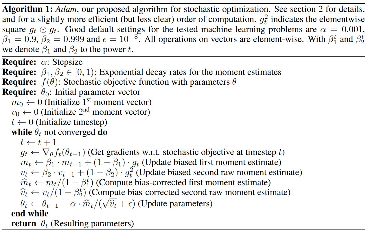
# Let there be Adam, the blessed optimizer and its buffers
learning_rate, beta1, beta2, eps_adam = 0.01, 0.85, 0.99, 1e-8
m = [0.0] * len(params) # first moment buffer
v = [0.0] * len(params) # second moment buffer

# Repeat in sequence
num_steps = 1000 # number of training steps
for step in range(num_steps):

    # Take single document, tokenize it, surround it with BOS special token on both sides
    doc = docs[step % len(docs)]
    tokens = [BOS] + [uchars.index(ch) for ch in doc] + [BOS]
    n = min(block_size, len(tokens) - 1)

    # Forward the token sequence through the model, building up the computation graph all the way to the loss
    keys, values = [[] for _ in range(n_layer)], [[] for _ in range(n_layer)]
    losses = []
    for pos_id in range(n):
        token_id, target_id = tokens[pos_id], tokens[pos_id + 1]
        logits = gpt(token_id, pos_id, keys, values)
        probs = softmax(logits)
        loss_t = -probs[target_id].log()
        losses.append(loss_t)
    loss = (1 / n) * sum(losses) # final average loss over the document sequence. May yours be low.

    # Backward the loss, calculating the gradients with respect to all model parameters
    loss.backward()

    # Adam optimizer update: update the model parameters based on the corresponding gradients
    lr_t = learning_rate * (1 - step / num_steps) # linear learning rate decay
    for i, p in enumerate(params):
        m[i] = beta1 * m[i] + (1 - beta1) * p.grad
        v[i] = beta2 * v[i] + (1 - beta2) * p.grad ** 2
        m_hat = m[i] / (1 - beta1 ** (step + 1))
        v_hat = v[i] / (1 - beta2 ** (step + 1))
        p.data -= lr_t * m_hat / (v_hat ** 0.5 + eps_adam)
        p.grad = 0

    print(f"step {step+1:4d} / {num_steps:4d} | loss {loss.data:.4f}", end='\r')

해당 부분은 학습을 수행하기 위한 부분인데 먼저 자주 쓰이는 optimizer인 Adam을 직접 구현한 모습이다. 일전에 모든 params를 flatten해 놓았기 때문에 반복문 하나로 gradient를 초기화할 수 있다. learning_rate는 step이 증가할수록 감소하게 설정하였다.

	# Adam optimizer update: update the model parameters based on the corresponding gradients
    lr_t = learning_rate * (1 - step / num_steps) # linear learning rate decay
    for i, p in enumerate(params):
        m[i] = beta1 * m[i] + (1 - beta1) * p.grad
        v[i] = beta2 * v[i] + (1 - beta2) * p.grad ** 2
        m_hat = m[i] / (1 - beta1 ** (step + 1))
        v_hat = v[i] / (1 - beta2 ** (step + 1))
        p.data -= lr_t * m_hat / (v_hat ** 0.5 + eps_adam)
        p.grad = 0

num_steps는 1000으로 설정하였다. num_steps만큼 반복문을 돌아가며 shuffle된 docs에서 이름을 순서대로 뽑아서 학습하게 되는데, 전체 이름이 32000개정도이므로 1/32 epoch정도 학습하는 셈이다.
이름의 앞뒤에 BOS토큰을 추가한다.
n은 학습을 위해 모델이 생성할 글자의 개수인데 block_size를 최대 단어의 길이보다 크게 설정하였으므로 학습하는 단어의 길이 -1만큼 반복하게 된다. -1인 이유는 transformer는 next token prediction이므로 토큰의 길이가 6이면 예측은 5번 수행할 수 있기 때문이다.
반복문을 돌아가며 학습하게 되는데 정답은 다음에 올 토큰이다. loss는 cross entropy를 사용한 것을 확인할 수 있다. 최종 loss는 average형태이다.
그 다음에 loss.backward를 수행하고 optimizer를 업데이트하고 gradient를 초기화한다.
관습적인 순서와는 다른데 미리 0으로 초기화하고 다음 for문으로 들어간다라고 보면 된다. 핵심은 zero_grad상태에서 loss.backward를 수행하고 결과를 optimizer update에 반영하는 것이다.

optimizer.zero_grad() -> loss.backward() -> optimizer.step() (o)
loss.backward() -> optimizer.step() -> optimizer.zero_grad() (o)
loss.backward() -> optimizer.zero_grad() -> optimizer.step() (x)

실행하면 loss가 의미있게 떨어진다라는 느낌을 받기는 어려운데 이는 batch size가 1이기 때문에 어려운 이름(ex. xzavier)의 경우 잘 못 맞힐 수 있다. 또한 모델 구조도 간단하고 1epoch도 보지 못했기 때문에 loss보다는 GPT의 동작 원리를 이해하는 데에 조금 더 집중하는 것이 적절할 것 같다.

# Inference: may the model babble back to us
temperature = 0.5 # in (0, 1], control the "creativity" of generated text, low to high
print("\n--- inference (new, hallucinated names) ---")
for sample_idx in range(20):
    keys, values = [[] for _ in range(n_layer)], [[] for _ in range(n_layer)]
    token_id = BOS
    sample = []
    for pos_id in range(block_size):
        logits = gpt(token_id, pos_id, keys, values)
        probs = softmax([l / temperature for l in logits])
        token_id = random.choices(range(vocab_size), weights=[p.data for p in probs])[0]
        if token_id == BOS:
            break
        sample.append(uchars[token_id])
    print(f"sample {sample_idx+1:2d}: {''.join(sample)}")

학습된 모델을 이용하여 추론하는 부분이다.
20개의 샘플을 생성할건데 이전 글자들의 정보를 기억할 KV cache를 초기화한다.
token_id는 BOS (27) 로 시작한다.
이름이 저장될 sample을 빈 리스트로 지정한다.
block_size의 길이만큼 반복문을 수행한다.
학습된 gpt모델에 현재 입력된 글자, 위치, keys, values를 전달한다.
모델은 logits을 반환하므로 softmax를 취해주는데 창의성을 조절하는 하이퍼파라미터인 temperature를 적용한다.

\[P_i = \frac{\exp(z_i / T)}{\sum_j \exp(z_j / T)}\]

T가 작으면 (0에 가까우면) 가장 점수가 높은 단어의 확률이 굉장히 높아지므로 일관된 답변을 내놓는다. T가 1보다 크면 지수함수의 기울기가 약화되므로 각 logits의 차이가 없고 조금 더 랜덤한 글자가 선택될 수 있다.
Temperature가 적용된 확률분포에 따라 랜덤하게 하나를 선택한다.
만약 BOS(끝나는 토큰이면 반복문을 빠져나간다). 즉 최대 block_size(16) 의 길이를 가진 이름이 생성될 수 있는 것이다.

BOS->a->n->n->a->BOS

생성된 샘플 이름은 다음과 같다.

--- inference (new, hallucinated names) ---
sample  1: kamon
sample  2: ann
sample  3: karai
sample  4: jaire
sample  5: vialan
sample  6: karia
sample  7: yeran
sample  8: anna
sample  9: areli
sample 10: kaina
sample 11: konna
sample 12: keylen
sample 13: liole
sample 14: alerin
sample 15: earan
sample 16: lenne
sample 17: kana
sample 18: lara
sample 19: alela
sample 20: anton

만약 T=0.01이면 다음과 같다.

--- inference (new, hallucinated names) ---
sample  1: anan
sample  2: anan
sample  3: anan
sample  4: anan
sample  5: anan
...

물론 이 코드가 실제 GPT의 구현이 모두 포함된 것은 아니다. 실제로는 글자가 아닌 서브워드 단위로 사용되고 RoPE, MoE, RLHF, flash attention, CoT 등 디테일이 많다.
하지만 파일의 머리말 부분에서 “This file is the complete algorithm. Everything else is just efficiency.”라고 한 것처럼 핵심 원리를 이해하기에는 좋은 코드라 생각된다. 특히 단 200줄로 파이썬 내장 라이브러리로만 구현이 가능한 것은 정말 놀랍다.

Reference

• https://gist.github.com/karpathy/8627fe009c40f57531cb18360106ce95
• https://arxiv.org/pdf/1412.6980