RL Course by David Silver - Lecture 2: Markov Decision Process

Markov Processes

fully observable한 경우

대부분의 강화학습 문제는 일종의 MDP의 한 유형으로 공식화될 수 있다.

최적제어는 MDP의 확인인 continuods MDPs를 다룬다.

또한 partially observable 문제도 MDP로 변화될 수 있다.

Bandits(팔이 여러개인 슬롯머신, 각 선택은 즉시 보상을 주고 미래에는 영향x)는 상태가 1개인 MDP이다.

복습) Markov Property: 다음에 일어날 일은 오직 현재 상태에만 의존하고 그 이전에 있었던 모든 일과는 관계없음

\[\mathbb{P}[S_{t+1} \mid S_t] = \mathbb{P}[S_{t+1} \mid S_1, \ldots, S_t]\]

State Transition Matrix

Markov state $s$, successor state $s’$ (후속 상태)일때, 상태 전이 확률

\[\mathcal{P}_{ss'} = \mathbb{P}[S_{t+1} = s' \mid S_t = s]\] \[\mathcal{P}=\text{from }\begin{bmatrix} \mathcal{P}_{11} & \cdots & \mathcal{P}_{1n} \\ \vdots & \ddots & \vdots \\ \mathcal{P}_{n1} & \cdots & \mathcal{P}_{nn} \end{bmatrix}\]

상태에서 다음 상태가 될 확률. 각 행의 합은 1이 된다.

Markov Process는 반복적으로 샘플링하는 프로세스이다 (memoryless random process)

ex. Markov property를 가진 무작위 상태 시퀀스 $S_1$, $S_2$, …

Definition) A Markov Process (or Markov Chain) is a tuple $\langle \mathcal{S}, \mathcal{P} \rangle$

• $\mathcal{S}$ is a (finite) set of states: 상태공간
• $\mathcal{P}$ is a state transition probability matrix: 전이확률

\[\mathcal{P}_{ss'} = \mathbb{P}\left[ S_{t+1} = s' \mid S_t = s \right]\]

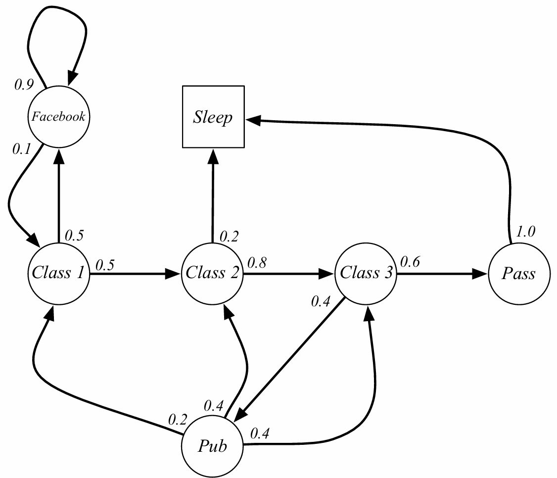
학생들이 3번의 수업을 듣고 pass한 후에 sleep까지 간다고 가정. sleep state는 markov process의 최종 상태

샘플 에피소드 (시퀀스에 대한 확률 분포로 추출된 무작위 시퀀스)

• C1 C2 C3 Pass Sleep
• C1 FB FB C1 C2 Sleep
• C1 C2 C3 Pub C2 C3 pass Sleep
• 정의상 추출하는 샘플은 유한한 길이를 가진다

	C1	C2	C3	Pass	Pub	Facebook	Sleep
C1		0.5				0.5
C2			0.8				0.2
C3				0.6	0.4
Pass							1.0
Pub	0.2	0.4	0.4
Facebook	0.1					0.9
Sleep							1

Q: 이러한 과정에서 만약 확률이 변한다면? ex. 페이스북 접속시마다 확률 감소

A: 2가지 방법이 있다. 1)non stationary MDP 사용 2) 비정상적인 거동으로 인해 더 복잡한 markov process를 구축. ex 페이스북 타이머 도입. 단순한 예제일 뿐 복잡할 수 있다.

Markov Reward Process

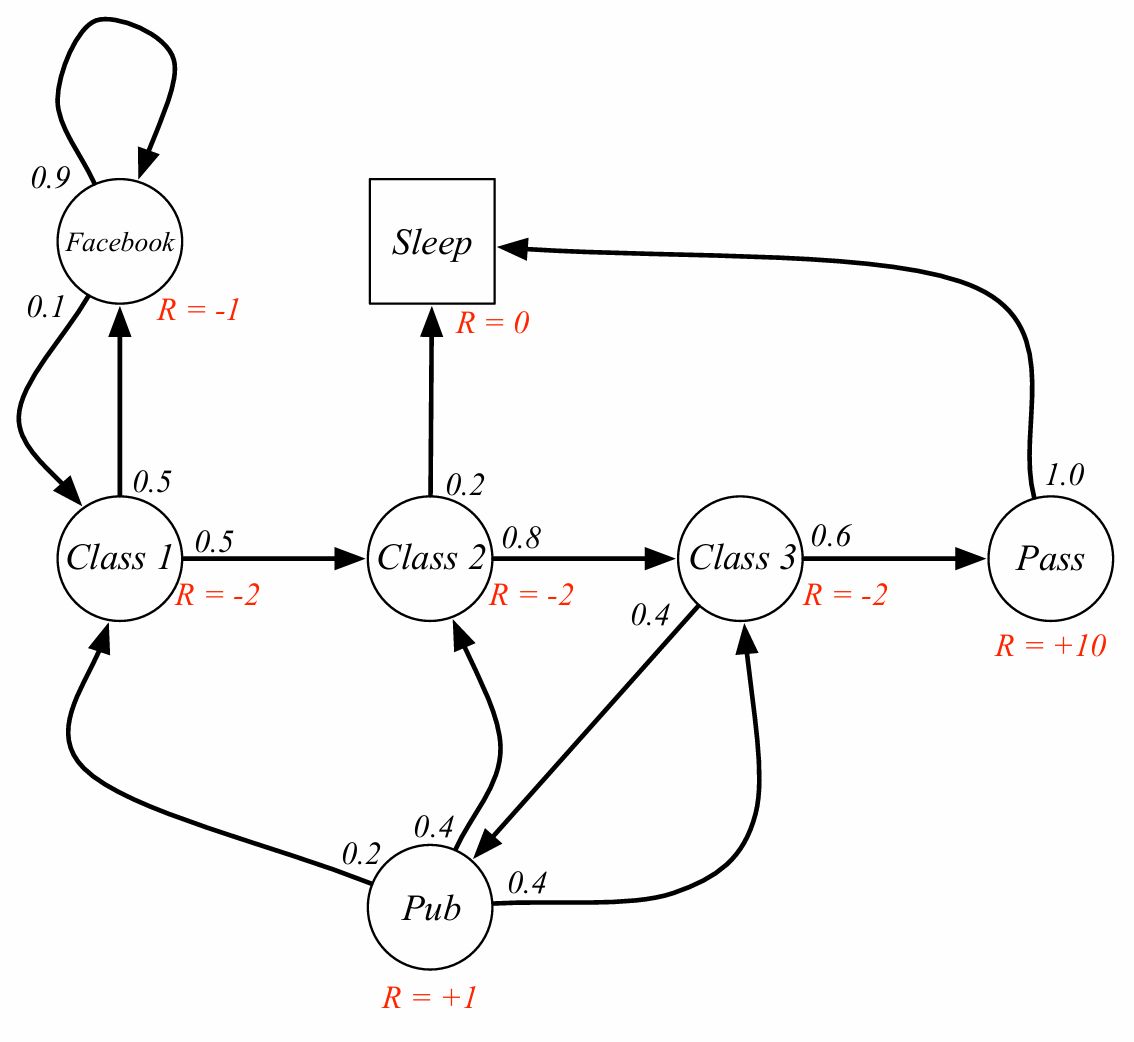
Markov reward process는 value가 있는 markov chain이다.

Definition) A Markov Reward Process is a tuple $\langle \mathcal{S}, \mathcal{P}, \mathcal{R}, \gamma \rangle$

• $\mathcal{S}$ is a (finite) set of states: 상태공간
• $\mathcal{P}$ is a state transition probability matrix: 전이확률
• $\mathcal{R}$ is a reward function: 그 상태에서 얻는 순간 보상
• $\gamma$ is discount factor, $\gamma$는 0~1사이의 값

\[\mathcal{P}_{ss'} = \mathbb{P}\left[ S_{t+1} = s' \mid S_t = s \right]\] \[\mathcal{R}_{s} = \mathbb{E}\left[ R_{t+1} \mid S_t = s \right]\]

Definition) The return $G_t$ is the total discounted reward from time-step $t$.(감가율 적용 시간보상 총합) G = Goal, finite하게 표현하기 위해 discount 적용. 이는 한 샘플에서의 값. 0에 가까운 값이면 현재 중시, 1에 가까운 값이면 미래 중시

\[G_t = R_{t+1} + \gamma R_{t+2} + \cdots = \sum_{k=0}^{\infty} \gamma^k R_{t+k+1}\]

왜 discount를 적용하는가?

• 수학적으로 편리
• infinite return 회피
• 금융 분야에서는 즉각적인 보상이 지연된 보상보다 가치 높음(현재의 돈의 가치가 미래다 높다)
• 동물/인간 행동은 즉각적인 보상 선호

Value function: 상태 $s$에서의 장기적인 가치

Definition) MRP의 상태 가치함수 $v(s)$는 상태 $s$에서의 기대값

\[v(s) = \mathbb{E}\left[ G_{t} \mid S_t = s \right]\]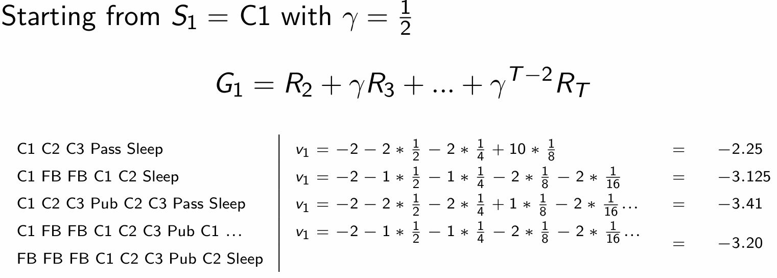

현재 상태의 가치를 어떻게 추정하는가? 여러 개 샘플링해서 평균을 취할 수 있다.

벨만 방정식 (for MRPs)

value function은 2가지 요소로 분해될 수 있다.

즉각적 보상 $R_{t+1}$, 감가율 적용된 후속 보상 $\gamma v(S_{t+1})$

\[\begin{aligned} v(s) &= \mathbb{E}[G_t \mid S_t = s] \\ &= \mathbb{E}[R_{t+1} + \gamma R_{t+2} + \gamma^2 R_{t+3} + \cdots \mid S_t = s] \\ &= \mathbb{E}[R_{t+1} + \gamma (R_{t+2} + \gamma R_{t+3} + \cdots) \mid S_t = s] \\ &= \mathbb{E}[R_{t+1} + \gamma G_{t+1} \mid S_t = s] \\ &= \mathbb{E}[R_{t+1} + \gamma v(S_{t+1}) \mid S_t = s] \end{aligned}\]

** 여기에서 t+1시점의 보상으로 표기된 것은 관례 중 하나이며 관점의 차이(인덱싱)

\[v(s)=\mathbb{E}[R_{t+1}+\gamma v(S_{t+1}) \mid S_t=s]\]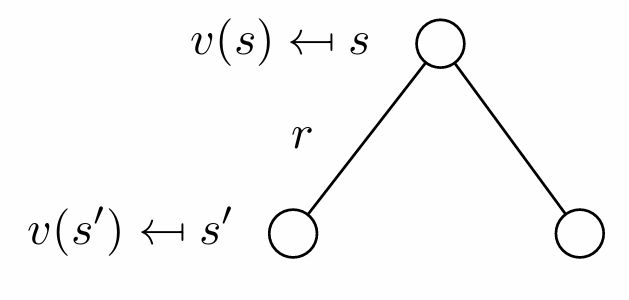

그림: 백업 다이어그램 \[v(s)=\mathcal{R}_s+\gamma\sum_{s'\in\mathcal{S}}\mathcal{P}_{ss'}\,v(s')\]

두번째 식은 재귀적 정의: 상태 $s$의 가치는 즉시 받는 보상 + 다음에 갈 수 있는 모든 상태 $s’$의 가치 $v(s’)$을 전이 확률로 가중 평균한 값의 합이다. 이 구조로 dynamic programming, value iteration, policy iteration이 가능해진다.

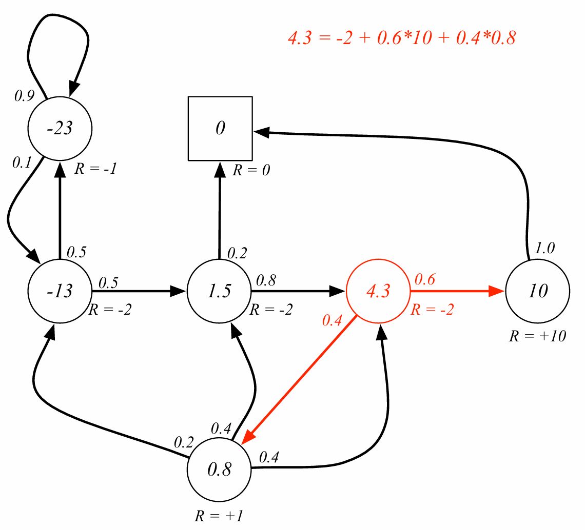
벨만 방정식은 분기 다음 상태만 고려한다. 감가율을 1이라고 가정하면 즉시 보상 -2에 10으로 갈 확률이 0.6, 0.8로 갈 확률이 0.4이므로 -2+6+0.32=4.32가 된다. 위 그림은 소수점 1자리까지 표시한 것으로 보인다.

사실 모든 값을 정확히 구하려면 연립방정식의 형태로 구성하거나 보상을 0으로 초기설정한 후에 반복계산으로 구해야 한다.

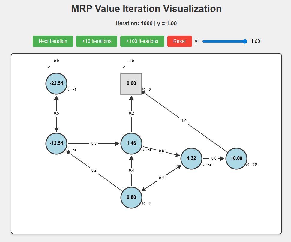
실제로 코드를 통해 1000회 반복해 보면 아래와 같은 값으로 수렴하는 것을 볼 수 있다.

해당 코드는 https://github.com/soribido/Study-Practice/blob/main/Reinforcement%20Learning/mrp_interactive.html 에서 확인할 수 있다.

벨만 방정식은 행렬을 통해 간결하게 나타낼 수도 있다. (가치=현재보상 + 감가율$\cdot$전이행렬$\cdot$가치)

\[\mathbf{v} = \mathcal{R} + \gamma \mathcal{P}\mathbf{v}\]

$v$는 상태별로 하나의 항목이 있는 열 벡터이다. 각 가치, 전이행렬 원소는 가능한 모든 상태 공간에 대해 정의된다.

\[\begin{bmatrix} v(1) \\ \vdots \\ v(n) \end{bmatrix} = \begin{bmatrix} \mathcal{R}_1 \\ \vdots \\ \mathcal{R}_n \end{bmatrix} + \gamma \begin{bmatrix} P_{11} & \cdots & P_{1n} \\ \vdots & \ddots & \vdots \\ P_{n1} & \cdots & P_{nn} \end{bmatrix} \begin{bmatrix} v(1) \\ \vdots \\ v(n) \end{bmatrix}\]

벨만 방정식은 선형 방정식으로 직접 풀 수 있다. (역행렬을 구할 수 있을만큼 충분히 작다면)

\[\begin{aligned} \mathbf{v} &= \mathcal{R} + \gamma \mathcal{P}\mathbf{v} \\ (\mathbf{I} - \gamma \mathcal{P})\,\mathbf{v} &= \mathcal{R} \\ \mathbf{v} &= (\mathbf{I} - \gamma \mathcal{P})^{-1}\mathcal{R} \end{aligned}\]

역행렬 계산은 $n$개의 상태에 대해 $O(n^{3})$의 시간복잡도를 지닌다. 따라서 실용적인 방안은 아니다. Large MDP에서 이를 계산할 수 있는 iterative 방법들이 존재한다. (Dynamic programming, Monte-Carlo evaluation, Temporal-Difference learning)

Markov Decision Process

Markov decision process는 MRP에 decision이 추가된 형태이다.

Definition) A Markov Decision Process is a tuple $\langle \mathcal{A},\mathcal{S}, \mathcal{P}, \mathcal{R}, \gamma \rangle$

• $\mathcal{S}$ is a (finite) set of states: 상태공간
• $\mathcal{A}$ is a (finite) set of states: 행동 공간 (action space)
• $\mathcal{P}$ is a state transition probability matrix: 전이확률
• $\mathcal{R}$ is a reward function: 그 상태에서 얻는 순간 보상
• $\gamma$ is discount factor, $\gamma$는 0~1사이의 값

\[\mathcal{P}^{a}_{ss'} = \mathbb{P}\left[ S_{t+1} = s' \mid S_t = s, A_t = a \right]\] \[\mathcal{R}^{a}_{s} = \mathbb{E}\left[ R_{t+1} \mid S_t = s, A_t = a \right]\]

결정 과정을 통해 보상을 최대화

Definition) A policy $\pi$ is a distribution over actions given states.

주어진 행동에 따른 확률 분포이다. ex) 특정 상태에서 ~로 갈 확률 0.9, 0.1 등

\[\pi(a \mid s) = \mathbb{P}\left[ A_{t}=a \mid S_{t} = s\right]\]

정책은 에이전트의 행동을 정의한다.

MDP 정책은 현재 상태에 의존한다 (not history)

MDP 정책은 stationary하다. (time-independent)

$A_t \sim \pi(\cdot \mid S_t), \forall t > 0$ 모든 시점 $t$에서 행동 $A_t$는 현재 상태 $S_t$에 조건부인 정책 $\pi$로 부터 샘플링된다.

예시)

\[\pi(\cdot \mid S_t)= \begin{cases} \Pr(A_t = a_1 \mid S_t) = 0.2 \\ \Pr(A_t = a_2 \mid S_t) = 0.5 \\ \Pr(A_t = a_3 \mid S_t) = 0.3 \end{cases}\]

Q) 왜 보상이 없는가?

A) markov process에서 s가 현재 상태부터 이후의 과정을 완벽하게 나타냄

Given an MDP $\mathcal{M}=\langle \mathcal{S}, \mathcal{A}, \mathcal{P}, \mathcal{R}, \gamma \rangle$ and a policy $\pi$,

the state sequence $S_1, S_2, \ldots$ is a Markov process $\langle \mathcal{S}, \mathcal{P}^\pi \rangle$.

• 왜? 정책이 고정되면 행동은 자유 변수가 아니라 다음 상태로의 확률이 자동으로 결정되어 markov chain이 된다. (행동이 평균 처리된다)

The state and reward sequence $S_1, R_2, S_2, \ldots$ is a Markov reward process $\langle \mathcal{S}, \mathcal{P}^\pi, \mathcal{R}^\pi, \gamma \rangle$, where

\[\mathcal{P}^\pi_{s,s'} = \sum_{a \in \mathcal{A}} \pi(a \mid s)\,\mathcal{P}^a_{ss'}\]

(정책 하에서의 전이 확률)

\[\mathcal{R}^\pi_s = \sum_{a \in \mathcal{A}} \pi(a \mid s)\,\mathcal{R}^a_s\]

(정책 하에서의 평균적으로 받는 즉시 보상)

Value function

Definition) The state-value function $v_\pi(s)$ of an MDP is the expected return starting from state $s$, and then following policy $\pi$.

상태가치함수: 상태 $s$에서 시작해서 그 이후에 정책 $\pi$를 그대로 따르면 앞으로 얻을 누적 보상의 기댓값 (이 상태의 가치는 얼마인가 (모든 행동을 샘플링 했을 때))

\[v_\pi(s) = \mathbb{E}_\pi \left[ G_t \mid S_t = s \right]\]

Definition) The action-value function $q_\pi(s,a)$ is the expected return starting from state $s$, taking action $a$, and then following policy $\pi$.

행동가치함수: 상태 $s$에서 시작해서 행동 $a$를 할 때 그 다음부터 정책 $\pi$를 따를 때 앞으로 얻을 누적 보상의 기댓값 (이 상태에서 이행동을 하는 것의 가치는 얼마인가)

\[q_\pi(s,a) = \mathbb{E}_\pi \left[ G_t \mid S_t = s, A_t = a \right]\]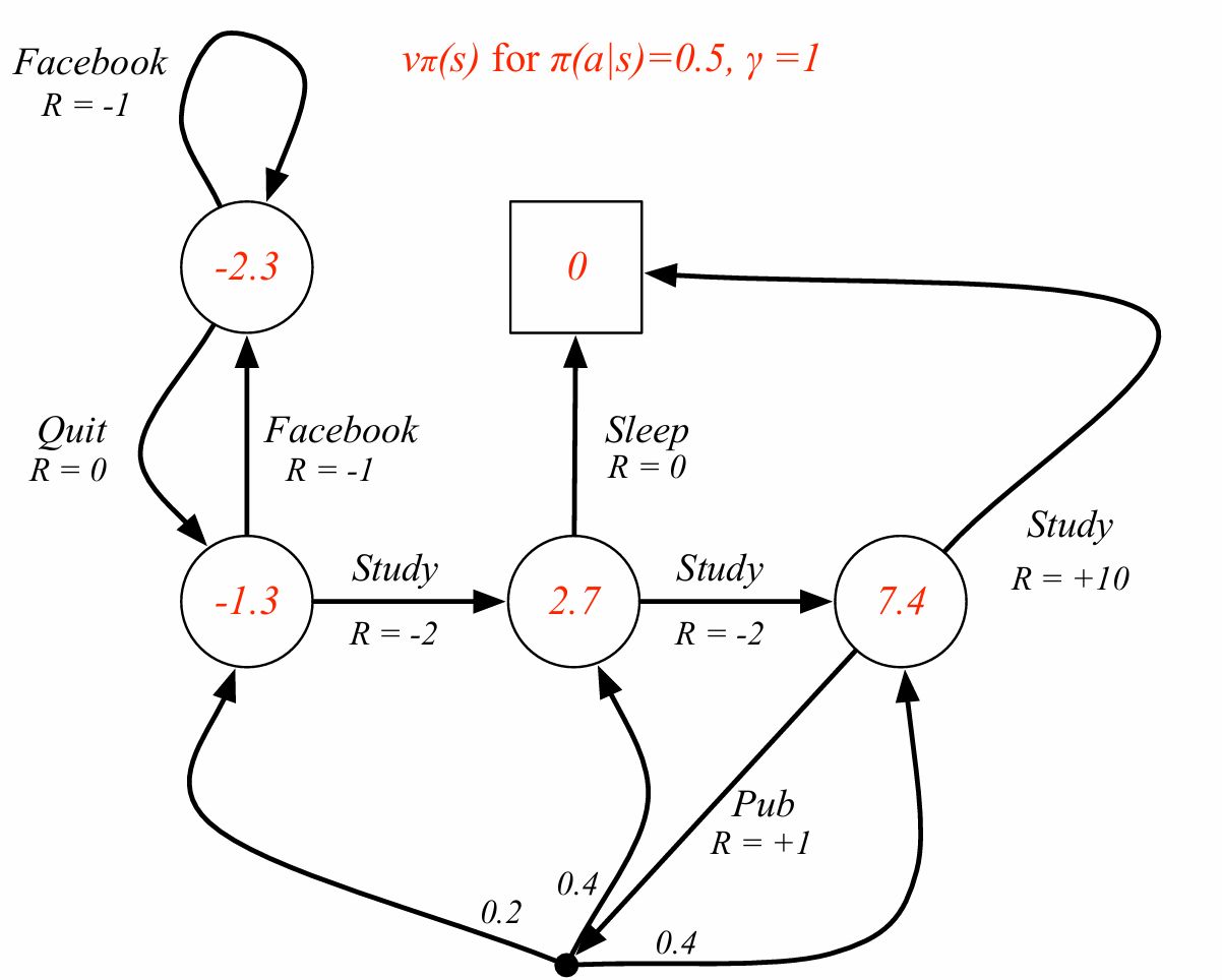

상태가치함수는 다시 현재 보상과 감가율을 적용한 다음 상태의 가치의 합으로 분해될 수 있다.

\[v_\pi(s)=\mathbb{E}_\pi \left[R_{t+1} + \gamma v_\pi(S_{t+1})\mid S_t = s\right]\]

행동가치함수 역시 비슷하게 분해 가능하다. 행동을 하고 도달을 한 상태의 상태가 가치가 얼마인지 알 수 있다.

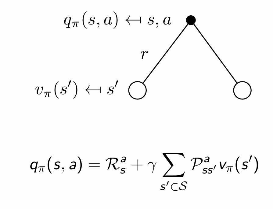
\[q_\pi(s,a)=\mathbb{E}_\pi \left[R_{t+1} + \gamma q_\pi(S_{t+1}, A_{t+1})\mid S_t = s, A_t = a\right]\]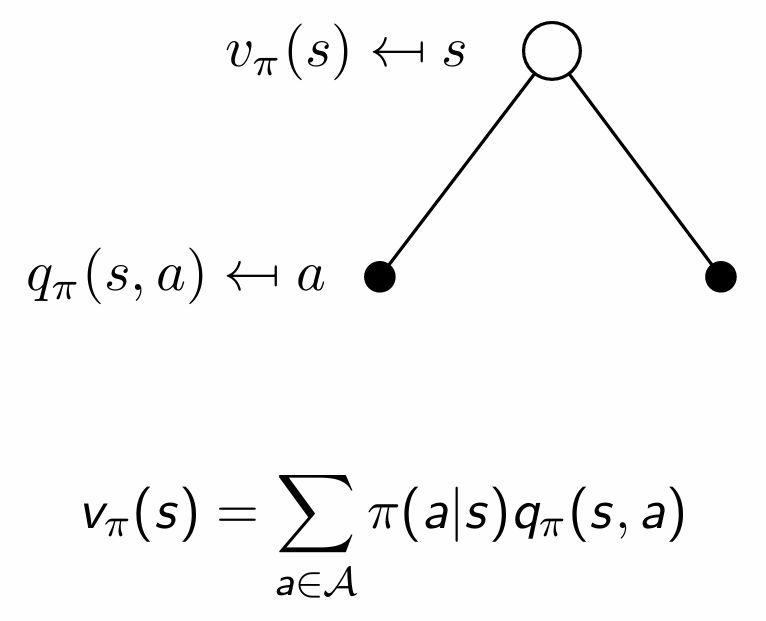

흰 원: state / 검은 원: action

\[q_\pi(s,a)=\mathbb{E}_\pi \left[R_{t+1} + \gamma q_\pi(S_{t+1}, A_{t+1})\mid S_t = s, A_t = a\right]\]

이에 대한 변환 과정이 강의에 없는데 어떻게 바뀌는지 이해하기 위해서는 기대값의 정의 및 성질을 활용해야 한다.

• $\mathbb{E}[X] = \sum_i x_i P(X = x_i)$ (이산 확률변수 정의)
• $\mathbb{E}[X+Y]=\mathbb{E}[X]+\mathbb{E}[Y]$ (선형)
• $\displaystyle \mathbb{E}[X \mid Y] = \sum_{z} P(Z = z \mid Y)\mathbb{E}[X \mid Y, Z = z]$ (전체기대의 법칙)

\[q_\pi(s,a)=\mathbb{E}_\pi \left[R_{t+1} \mid S_t = s, A_t = a\right]+\gamma\mathbb{E}_\pi \left[q_\pi(S_{t+1}, A_{t+1})\mid S_t = s, A_t = a\right]\]

먼저 원래 행동 가치함수에 대한 식을 다음상태 $s’$에 대한 확률의 합으로 표현할 수 있다. (전체기대의 법칙) action이 정해지더라도 다음 state에서는 랜덤이다.

\[\displaystyle q_\pi(s,a)=\sum_{s'}P(S_{t+1}=s'\mid S_t=s,A_t=a)\mathbb{E}_\pi[R_{t+1}+\gamma q_\pi(S_{t+1},A_{t+1})\mid S_t=s,A_t=a,S_{t+1}=s']\]

다음으로, 보상과 미래 가치를 분리한다.

\[\displaystyle q_\pi(s,a)=\sum_{s'}P(s'\mid s,a)\left(\mathbb{E}[R_{t+1}\mid s,a,s']+\gamma\mathbb{E}_\pi[q_\pi(S_{t+1},A_{t+1})\mid S_{t+1}=s']\right)\] \[\mathbb{E}[R_{t+1}\mid s,a,s']=\mathcal{R}_s^a\] \[P(s'\mid s,a)=\mathcal{P}_{ss'}^a\] \[\mathbb{E}_\pi[q_\pi(S_{t+1},A_{t+1})\mid S_{t+1}=s']=v_\pi(s')\]

위 식들로 단순화하면 아래와 같은 식을 얻을 수 있다.

\[q_\pi(s,a)=\mathcal{R}_s^a+\gamma\sum_{s'\in\mathcal{S}}\mathcal{P}_{ss'}^a\,v_\pi(s')\]

이는 기대값과 다르게 우리가 알고리즘으로 계산할 수 있는 형태이다.

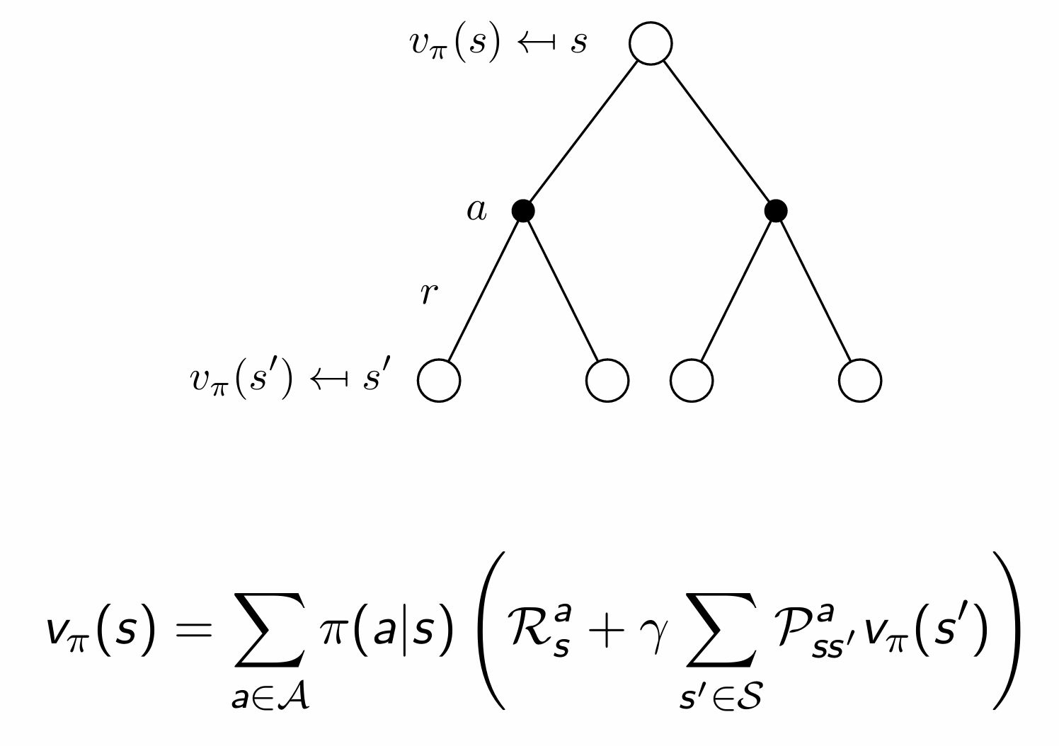
$\displaystyle v_\pi(s)=\sum_{a\in\mathcal{A}}\pi(a\mid s)q_\pi(s,a)$ 이므로 행동가치함수를 위에서 구한 식으로 대체 가능하다.

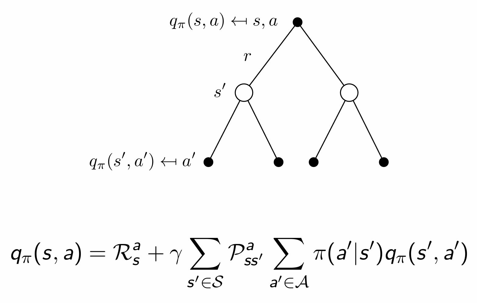
$\displaystyle v_\pi(s)=\sum_{a\in\mathcal{A}}\pi(a\mid s)q_\pi(s,a)$ 이므로 위에서 구한 식에 다시 상태가치함수를 대입하면 똑같이 얻을 수 있다. 의미적으로는 다음상태에서의 action, state들의 환경에 대해 평균, 정책에 대해 평균한 미래 가치를 더해준다는 뜻이다.

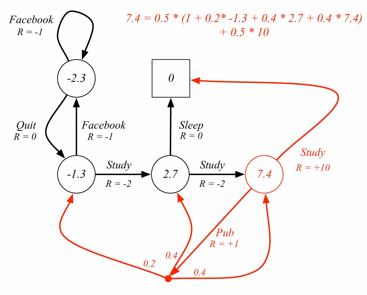
다시 student MDP문제로 돌아가자.

study, pub 분기 확률이 0.5라면 행동에 대한 가치는 0.5에 pub 즉시보상1, pub에서의 다음 state로 가는 action들의 평균 가치 합+ 0.5에 10이다. 여기에서 점은 decision이다. facebook이나 sleep에도 분기가 될수 있는 점이 있고 확률이 1인 것이다.

평균화된 형태의 식으로도 표현이 가능하다.

\[v_\pi=\mathcal{R}^\pi+\gamma\mathcal{P}^\pi v_\pi\] \[v_\pi=(I-\gamma\mathcal{P}^\pi)^{-1}\mathcal{R}^\pi\]

Optimal value function

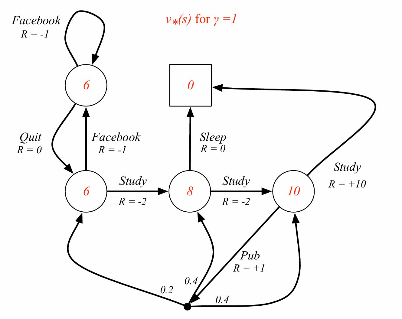
Definition) The optimal state-value function $v_*(s)$ is the maximum value function over all policies.

\[v_*(s) = \max_\pi v_\pi(s)\]

(최적 상태가치함수)

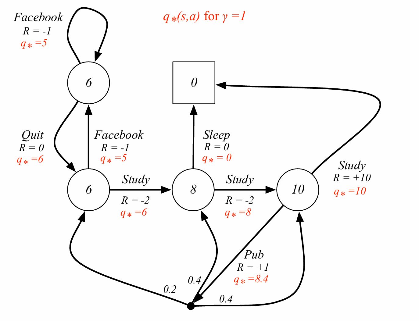
The optimal action-value function $q_*(s,a)$ is the maximum action-value function over all policies.

\[q_*(s,a) = \max_\pi q_\pi(s,a)\]

(최적 행동가치함수)

• The optimal value function specifies the best possible performance in the MDP.
• An MDP is solved when we know the optimal value function.
• $q_*$를 알면 MDP문제를 해결한 것이다. (왼쪽으로 가면 70 오른쪽으로 가면 80이면 오른쪽으로 가야 한다.)

Define a partial ordering over policies,

$\pi \succeq \pi’$ if $v_\pi(s) \ge v_{\pi’}(s), \forall s$ 모든 상태에서 가치가 큰 정책이 있다면 이 정책이 같거나 더 좋은 정책이다.

Theorem) For any Markov Decision Process,

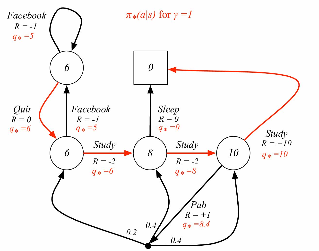
• There exists an optimal policy $\pi_\ast$ that is better than or equal to all other policies: $\pi_\ast \succeq \pi, \forall \pi$. 어떤 MDP든 다른 모든 정책보다 같거나 더 좋은 정책 $\pi_\ast$가 항상 적어도 1개 이상 존한다.
• All optimal policies achieve the optimal value function: $v_{\pi_\ast}(s) = v_\ast(s)$. 모든 최적 정책은 같은 상태가치를 만든다. 최적 정책이 여러 개 있을 수 있지만 만들어내는 상태 가치 함수는 동일하다.
• All optimal policies achieve the optimal action-value function: $q_{\pi_\ast}(s,a) = q_\ast(s,a)$. 모든 최적 정책은 같은 행동가치를 만든다.

\[\pi_*(a \mid s)= \begin{cases} 1 & \text{if } a=\arg\max_{a\in\mathcal{A}} q_*(s,a) \\ 0 & \text{otherwise} \end{cases}\]

가장 좋은 최적 정책이 있으면 결정론적으로 고르면 된다.

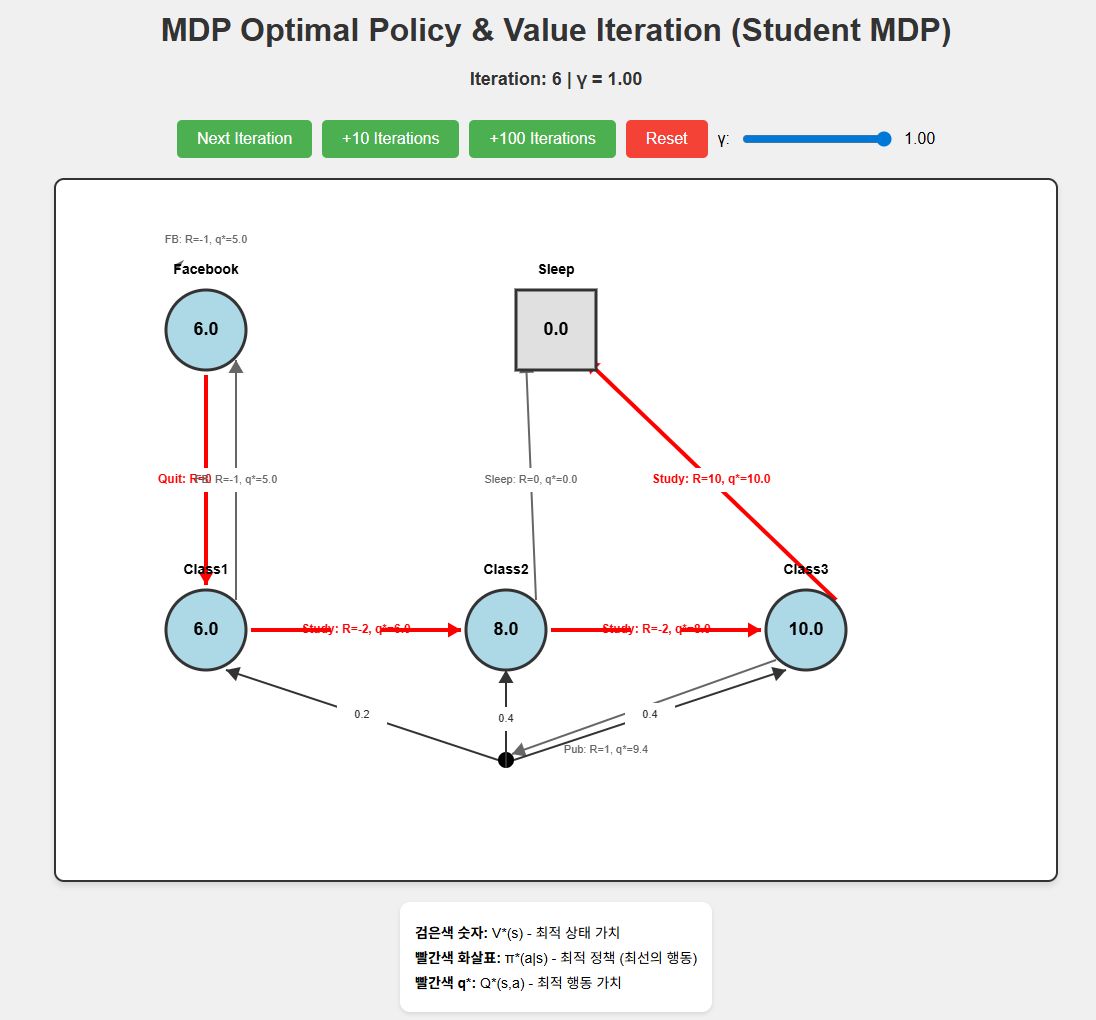
iteration 5정도에서 수렴하는 것을 확인할 수 있고 다른 점은 강의자료에서 pub에서의 $q_*$가 8.4라고 나오지만 실제로 반복 실행을 수행하면 9.4로 수렴하는 것을 확인할 수 있다.

해당 코드는 https://github.com/soribido/Study-Practice/blob/main/Reinforcement%20Learning/mdp_optimal_policy.html 에서 확인할 수 있다.

즉각보상 + 다음 상태 분기의 가치의 식을 적용하면

\[\displaystyle q_*(s,a)=\mathcal{R}_s^a+\gamma\sum_{s'\in\mathcal{S}}\mathcal{P}_{ss'}^a\,v_*(s')\]

1+ 1.0(감가율) x (0.2 x 6 + 0.4 x 8 + 0.4 x 10) = 1+8.4이므로 9.4가 맞다.

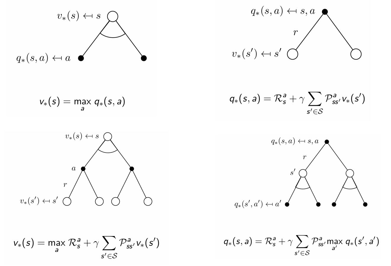
분기에 대해 개념적으로 생각하면 위 그림과 같은 식을 얻을 수 있다.

\[\displaystyle v_*(s)=\max_a\mathcal{R}_s^a+\gamma\sum_{s'\in\mathcal{S}}\mathcal{P}_{ss'}^a\,v_*(s')\] \[\displaystyle q_*(s,a)=\mathcal{R}_s^a+\gamma\sum_{s'\in\mathcal{S}}\mathcal{P}_{ss'}^a\max_{a'}q_*(s',a')\]

이 식을 bellman optimality equation이라 하며 엄밀한 bellman equation은 앞서 정의한 식이지만 일반적으로 벨만 방정식이라 하면 이 식을 의미한다.

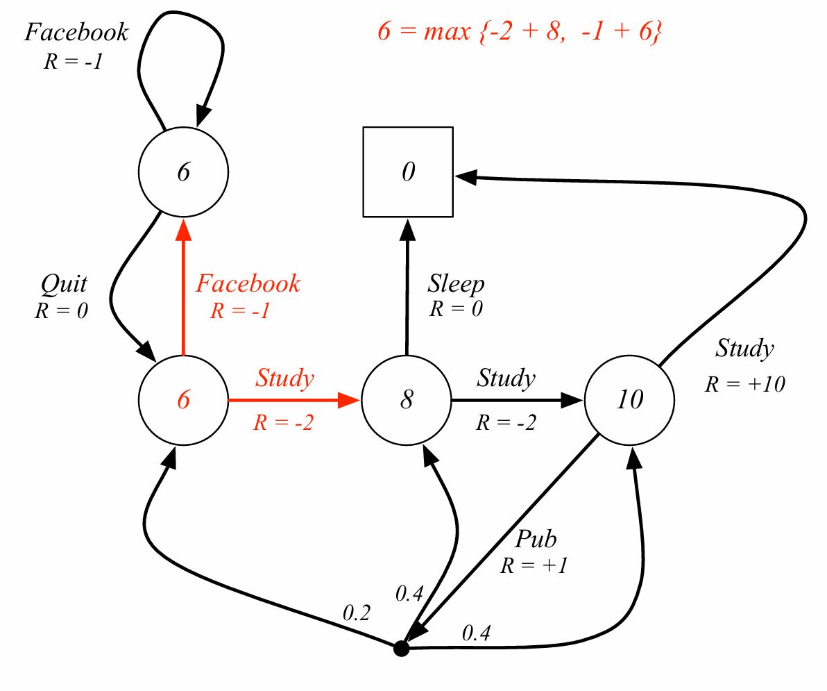
상태가치 6이라는 숫자는 다음 상태를 봤을때 6,5로 갈라지며 그 중 최대값(모든 행동에 대한 최대값)인 6이 되는 것이다.

Bellman optimality equation은 non-linear한 경우가 있는데 이런 경우는 general solution(역행렬을 통해 구함)이 존재하지 않고 반복적인 방법을 통해 해결해야 한다.

• Value Iteration
• Policy Iteration
• Q-learning
• Sarsa

Q) state가 많은 경우에는 MDP 보상을 어떻게 모델링하는가?

A) 환경 동역학으로부터 계산할 수 있는 보상함수 설계

Reference

https://www.youtube.com/watch?v=lfHX2hHRMVQ&list=PLqYmG7hTraZDM-OYHWgPebj2MfCFzFObQ&index=2